sketch
Copyright © 2005, 2006, 2007, 2008 Eugene K. Ressler.
This manual is for sketch, version 0.2 (build 131),
Saturday, August 09, 2008, a program that converts descriptions of simple
three-dimensional scenes into static drawings. This version generates
PSTricks or PGF/TikZ code suitable for use with the
TeX document processing system.
Sketch is free software; you can redistribute it and/or modify
it under the terms of the GNU General Public License as published by
the Free Software Foundation; either version 3, or (at your option)
any later version.
Sketch is distributed in the hope that it will be useful, but WITHOUT ANY WARRANTY; without even the implied warranty of MERCHANTABILITY or FITNESS FOR A PARTICULAR PURPOSE. See the GNU General Public License for more details.
You should have received a copy of the GNU General Public License
along with sketch; see the file COPYING.txt. If not, see
http://www.gnu.org/copyleft.
--- The Detailed Node Listing ---
About sketch
Introduction by example
Swept objects
Input language
Basics
Literals
Arithmetic expressions
Options
Point lists
Drawables
Sweeps
Definitions
Global environment
Building a drawing
Caveats
Hidden surface removal and polygon splitting
Sketch is a small, simple system for producing line drawings of
two- or three-dimensional objects and scenes. It began as a way to
make illustrations for a textbook after we could find no suitable
tool for this purpose. Existing scene processors emphasized GUIs
and/or photo-realism, both un-useful to us. We wanted to produce
finely wrought, mathematically-based illustrations with no extraneous
detail.
Sketch accepts a tiny scene description language and generates
PSTricks or TikZ/PGF code for LaTeX. The
sketch language is similar to PSTricks, making it easy
to learn for current PSTricks users. See
www.pstricks.de for information on PSTricks.
TikZ/PGF are also very similar except for details of syntax.
See
http://sourceforge.net/projects/pgf. One can easily lay raw
PSTricks or TikZ/PGF output over, in, or under
sketch drawings, providing the full power of LaTeX text and
mathematics formatting in a three-dimensional setting.
Send bug reports and suggestions to [email protected]. We will try to respond, but can't promise. In any event, don't be offended if a reply is not forthcoming. We're just busy and will get to your suggestion eventually.
For bugs, attach a sketch input file that causes the bad
behavior. Embed comments that explain what to look for in
the behavior of sketch or its output.
A recommendation for improvement from one unknown person counts as one vote. We use overall vote tallies to decide what to do next as resources permit. We reserve the right to a assign any number of votes to suggestions from people who have been helpful and supportive in the past.
If you intend to implement an enhancement of your own, that's terrific! Consider collaborating with us first to see if we're already working on your idea or if we can use your work in the official release.
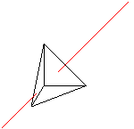
The sketch input language will seem familiar to users of the
PSTricks package for LaTeX. The following program draws a
triangular polygon pierced by a line.
  polygon(0,0,1)(1,0,0)(0,1,0)
  line(-1,-1,-1)(2,2,2)
The coordinate system is a standard right-handed Cartesian one.

The sketch program above is nearly the simplest one possible,
the equivalent of a “hello world”
program you might find at the start of a programming language text.
If it is saved in the file simple.sk, then the command
sketch simple.sk -o simple.texcreates a file simple.tex containing
PSTricks commands to
draw these objects on paper. The contents of simple.tex
look like this.
  \begin{pspicture}(-1,-1)(2,2)
  \pstVerb{1 setlinejoin}
  \psline(-1,-1)(.333,.333)
  \pspolygon[fillstyle=solid,fillcolor=white](0,0)(1,0)(0,1)
  \psline(.333,.333)(2,2)
  \end{pspicture}
The hidden surface algorithm
of sketch has split
the line into
two pieces and ordered the three resulting objects so that the correct
portion of the line is hidden.
If you've noticed that the projection we are using seems equivalent to erasing the z-coordinate of the three-dimensional input points, pat yourself on the back. You are correct. This is called a parallel projection. The z-coordinate axis is pointing straight out of the paper at us, while the x- and y-axes point to the right and up as usual.
The resulting picture file can be included in a LaTeX document with
\input{simple}. Alternately, adding the command line option
-T1
causes the pspicture to be wrapped in a short
but complete document, ready to run though LaTeX.
In a finished, typeset document, the picture looks like this. (The
axes have been added in light gray.)
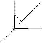
It is important to know that only the “outside”
of a polygon is
normally drawn. The outside is where the vertices given in the
polygon
command appear in counter-clockwise
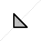
order. Thus, if the command above had been
polygon(0,1,0)(1,0,0)(0,0,1)the polygon would not appear in the picture at all. It would have been culled from the scene. This culling behavior may seem strange, but stay tuned.
Many PSTricks and TikZ/PGF options
work just fine in sketch. If generating PSTricks, the code
  polygon[fillcolor=lightgray,linewidth=3pt](0,0,1)(1,0,0)(0,1,0)
  line[linestyle=dotted](-1,-1,-1)(2,2,2)
produces
To produce TikZ/PGF, the corresponding code is
  polygon[fill=lightgray,line width=3pt](0,0,1)(1,0,0)(0,1,0)
  line[style=dotted](-1,-1,-1)(2,2,2)
  global { language tikz }
The final global
instructs sketch to produce TikZ/PGF code as output
rather than the default, PSTricks. Note that polygon
fill color and line style options both conform to TikZ
syntax rules. The remaining examples of this manual are in PSTricks
style.
Let's try something more exciting. Sketch has no notion of a
solid,
but polygonal faces
can be used to represent the
boundary of a solid. To the previous example, let's add three more
triangular polygons to make the faces of an irregular tetrahedron.
  % vertices of the tetrahedron
  def p1 (0,0,1) def p2 (1,0,0)
  def p3 (0,1,0) def p4 (-.3,-.5,-.8)

  % faces of the tetrahedron.
  polygon(p1)(p2)(p3) % original front polygon
  polygon(p1)(p4)(p2) % bottom
  polygon(p1)(p3)(p4) % left
  polygon(p3)(p2)(p4) % rear

  % line to pierce the tetrahedron
  line[linecolor=red](-1,-1,-1)(2,2,2)
This example uses definitions, which begin with
def.
These define or give names to points,
which are then available
as references
by enclosing the names in parentheses,
e.g. (foo).
The parentheses denote that the names refer to points; they are
required. There can be no
white space between them and the name.
As you can see, comments
start with % as in TeX and extend
to the end of the line (though # will work as well). White
space,
including spaces, tabs and blank lines, has no effect in the sketch
language.
If we look inside the TeX file produced by sketch, there
will be only three polygons. The fourth has been
culled because it is
a “back face”
of the tetrahedron, invisible to our view. It is
unnecessary, and so it is removed.
In some drawings, polygons act as zero-thickness solid surfaces with
both sides visible rather than as the faces of solid objects, where
back faces can be culled. For zero-thickness solids, culling
is a
problem. One solution is to use a pair of sketch polygons for
each zero-thickness face, identical except with opposite vertex
orders. This is unwieldy and expensive. A better way is to
set the sketch internal option cull to false in
the usual PSTricks manner.
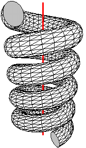
polygon[cull=false](p1)(p2)(p3)The following shows the same helix shape drawn first with cull=true (the default) and then cull=false.
We'll soon see how to produce these helixes with a few lines
of sketch language code.
It may be tempting to turn culling off gratuitously so that vertex order
can be ignored. This is not a good idea because output file size and
TeX and Postscript processing time both depend on the number of
output polygons. Culling usually improves performance by a factor of
two. On the other hand, globally setting cull=false is
reasonable while debugging. See Global options and
Limits on error detection.
We can add labels
to a drawing by using special
objects, which provide a way to embed raw LaTeX and PSTricks
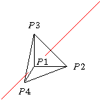
code. Adding this to the tetrahedron does the trick.
  special |\footnotesize
           \uput{2pt}[ur]#1{$P1$}
           \uput[r]#2{$P2$}
           \uput[u]#3{$P3$}
           \uput[d]#4{$P4$}|
    (p1)(p2)(p3)(p4)
Here is the result.
There are several details to note here. First, the quoting convention for the raw code is similar to the LaTeX \verb command. The first non-white space character following special is understood to be the quote character, in this case |. The raw text continues until this character recurs.
Second, the argument references
#1, #2, #3,
and #4 refer to points in the list that follow. This is
similar to TeX macro syntax. The transformed and two-dimensional
projections of these three-dimensional points are substituted
in the final output. An argument reference of the form #1-2
is replaced with the angle in degrees of the two-dimensional vector
that connects the projections of the two respective argument points,
here #1 and #2. The substituted angle is enclosed
in curly braces { }
By default, special objects are printed last, overlaying all
other objects in the scene. If you specify the internal option
lay=in, the hidden surface algorithm
considers the entire special object to be the first point
(#1) in the argument list. If that point is behind (of
smaller z-component than) any drawable, then the entire special
object is drawn before that drawable, so the drawable obscures parts of
the special object that overlaps it. In our example, p1 is
the front-most point in the scene (has the largest
z-component), so adding lay=in has no effect.
With option lay=under, a special is drawn before, hence
appears under any of the objects handled by the hidden surface
algorithm. This is how the light gray axes were added to the “hello
world” example Hello world.
Special objects are powerful, with many possible uses.
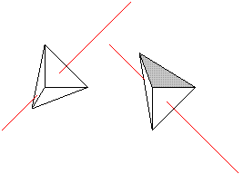
Now let's add a second copy of the pierced tetrahedron. We'll rotate the copy 90 degrees about the x-axis with the origin as center of rotation so we can see the back, then translate it to the right—in the positive x-direction—so it doesn't collide with the original. To help us see what's going on, make the back side gray.
  def pierced_tetrahedron {
    def p1 (0,0,1) def p2 (1,0,0)
    def p3 (0,1,0) def p4 (-.3,-.5,-.8)
    polygon(p1)(p2)(p3)                      % original
    polygon(p1)(p4)(p2)                      % bottom
    polygon(p1)(p3)(p4)                      % left
    polygon[fillcolor=lightgray](p3)(p2)(p4) % rear
    line[linecolor=red](-1,-1,-1)(2,2,2)
  }
  {pierced_tetrahedron}  % tetrahedron in original position
  put { rotate(90, (0,0,0), [1,0,0]) % copy in new position
        then translate([2.5,0,0]) } {pierced_tetrahedron}
Here the entire code of the previous example has been wrapped in a
definition by forming a block
with braces (a single item would not need them). The point
definitions nested inside the braces are lexically scoped.
Their meaning extends only to the end of the block. The outer
def is called a drawable
definition
because it describes something that can be drawn.
A drawable definition by itself causes nothing to happen until its
name is referenced. Drawable references must be enclosed in curly
braces, e.g. {foo}, with no intervening
white space. In the code
above, the first reference
{pierced_tetrahedron}
is a plain
one. Its effect is merely to duplicate the earlier drawing. Almost
any series of sketch commands stuff may be replaced
with def foo { stuff } {foo} without changing its meaning.
The put command supplies a second reference, this time with a transform applied first. The rotate transform turns the tetrahedron 90 degrees about the origin. The axis of rotation is the vector [1,0,0]. By the right hand rule, this causes the top of the tetrahedron to rotate toward the viewer and the bottom away. The rule receives its name from the following definition:
Right hand rule. If the right hand is wrapped around any axis with the thumb pointing in the axis direction, then the fingers curl in the direction of positive rotation about that axis.The translate transform moves the pyramid laterally to the right by adding the vector [2.5,0,0] to each vertex coordinate. The result is shown here.
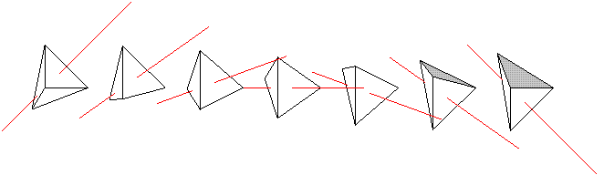
To draw seven instances of the tetrahedron, each differing from the last by the same transform, replace the last two commands of the previous example with
  repeat { 7, rotate(15, (0,0,0), [1,0,0]) % copy in new position
              then translate([2,0,0]) } {pierced_tetrahedron}
And the result....
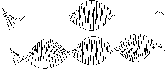
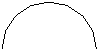
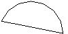
Many familiar shapes can be generated by sweeping simpler ones through
space and considering the resulting path, surface, or volume.
Sketch implements this idea in the sweep command.
  def n_segs 8
  sweep { n_segs, rotate(180 / n_segs, (0,0,0), [0,0,1]) } (1,0,0)
This code sweeps the point (1,0,0)
eight times by rotating it
180/8 = 22.5 degrees each time and connecting the resulting
points with line segments. The def used here is a
scalar definition.
References to
scalars have no enclosing brackets at all.
Sweeping a point makes a one-dimensional path, which is a polyline. Since we have swept with a rotation, the result is a circular arc. Here is what it looks like.
This is the first example we have seen of sketch arithmetic.
The expression 180 / n_segs causes the eight rotations to add
to 180. If you're paying attention, you'll have already noted that
there are nine points, producing eight line segments.
You can cause the swept point to generate a single polygon rather than a polyline by using the closure tag <> after the number of swept objects. Code and result follow
  def n_segs 8
  sweep { n_segs<>, rotate(180 / n_segs, (0,0,0), [0,0,1]) } (1,0,0)
Sweeping a polyline produces a surface composed of many faces. The unbroken helix in the example Helix with cull set false then true is produced by this code (plus a surrounding put rotation to make an interesting view; this has been omitted).
  def K [0,0,1]
  sweep[cull=false] {
    60,
    rotate(10, (0,0,0), [K]) then translate(1/6 * [K])
  } line[linewidth=2pt](-1,0)(1,0)
Again, 60 segments of the helix
are produced by connecting 61
instances of the swept line. Options
applied to the sweep, here
cull=false, are treated as options for the generated polygon
or polyline. Options of the swept line itself, here
linewidth=2pt, are ignored, though with a warning. This
def is a vector definition,
which must be referenced
with square brackets, e.g. [foo].
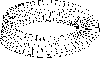
When the center point of rotation is omitted, the origin is assumed. When a point has only two coordinates, they are taken as x and y, with z=0 assumed. A toroid is therefore obtained with this code.
  def n_toroid_segs 20   def n_circle_segs 16
  def r_minor 1          def r_major 1.5
  sweep { n_toroid_segs, rotate(360 / n_toroid_segs, [0,1,0]) }
    sweep { n_circle_segs, rotate(360 / n_circle_segs, (r_major,0,0)) }
      (r_major + r_minor, 0)
For intuition, the idea of the code is to sketch a circle to the right
of the origin in the xy-plane, then rotate that circle “out of
the plane” about the y-axis to make the final figure. This
produces the following. (A view rotation and some axes have been
added.)
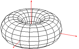
This example also shows that the swept object may itself be another
sweep.
In fact, it may be any sketch expression that results in
a list of one or more points or, alternately, a list of one or more
polylines and polygons. The latter kind of list can be created with a
{ }-enclosed block, perhaps following a
put or
repeat.
Sweeping a polygon creates a closed surface with polygons at the ends, which are just copies of the original, appropriately positioned. See Solid coil example. Options on the swept polygon, if they exist, are applied to the ends. Otherwise the sweep options are used throughout.
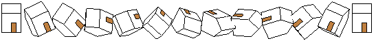
A polyline sweep with a closure tag creates another kind of closed surface. First, the polyline segments are connected by faces, just as without the closure tag. Then, each set of end points is joined to make a polygon, one for each end. A code for several views of a cylindrical prism follows.
  def n_cyl_segs 20  def n_views 5  def I [1,0,0]
  def endopts [fillcolor=lightgray]
  repeat { n_views, rotate(180/n_views, [I]) then translate([I] * 2.1) }
    sweep[endopts]{ n_cyl_segs<>, rotate(360/n_cyl_segs, [0,1,0]) }
      line[fillcolor=white](1,-1)(1,1)
It produces this drawing.
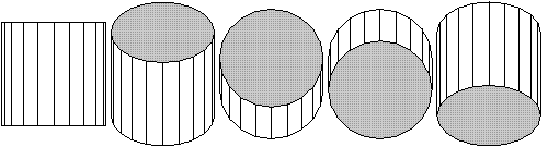
The options of the swept line, if any, are applied to the faces
produced by sweeping the line, but not the end polygons. Otherwise,
the sweep options are applied throughout.
The def in this example is an option definition.
References to options must be enclosed in square brackets, e.g.
[foo].
Happily, the syntax of sketch is such that
options references can never be confused with vector references. While
not apparent in this example, options references are useful when
defining many objects with a similar appearance.
The arithmetic [I] * 2.1 above hints at a larger truth.
Sketch operators work on scalars, vectors, points, and
transforms according to the general rules of affine algebra.
This can be helpful for setting up diagrams with computed geometry.
For example, if you have triangle vertices (p1) through
(p3) and need to draw a unit normal vector pointing out of
the center of the triangle, this code does the trick.
  def p1 (1,0,0)  def p2 (0,0.5,0)  def p3 (-0.5,-1,2)
  def O (0,0,0)
  def N unit( ((p3) - (p2)) * ((p1) - (p2)) )
  def n1 ((p1)-(O) + (p2)-(O) + (p3)-(O)) / 3 + (O)
  def n2 (n1)+[N]
  polygon(p1)(p2)(p3)
  line[arrows=*->](n1)(n2)
The first line computes the cross product of two edge vectors of the triangle and scales it to unit length. The second computes the average of the vertices. Note that subtraction and addition of the origin effectively convert vectors to points and vice versa. The line command draws the normal at the correct spot.

Two caveats regarding this example remain. First, the only way to use
PSTricks-style arrows is with arrows=.
The alternative syntax for PSTricks arrows is not allowed in
sketch. Second, you might like to eliminate the third
def and write instead the following.
line[arrows=*->](n1) (n1)+[N]This is not allowed. The point lists in drawables may consist only of explicit points or point references. You may, however, use arithmetic to calculate point components. The following works, though it's a little cumbersome.
line[arrows=*->](n1)((n1)'x+(N)'x, (n1)'y+(N)'y, (n1)'z+(N)'z)Obviously, the tick operator 'x extracts components of points and vectors.
This is not the end of the story on sweeps! We invite the reader into the main body of this documentation Sweeps to learn more.
Who knows where you'll finish?
This chapter describes the sketch input language in detail.
Sketch input is plain ASCII text, usually stored in an input
file.
It describes a scene,
so the sketch language is a scene description
language.
Sketch input is also declarative.
It merely
declares what the scene ought to look like when drawing is complete
and says very little about how sketch should do its work.
Sketch commands are not executed sequentially as in the usual
programming language. They merely contribute to that declaration.
A few syntactic details are important. Case is significant in the
sketch language. With a few exceptions, white space is not.
This includes line breaks.
Comments begin with % or # and extend to the end of the
line. You can disable a chunk of syntactically correct sketch
code by enclosing it in a def.
There is a simple “include file” mechanism.
The command
input{otherfile.sk}
causes the contents of otherfile.sk to be inserted as though
they were part of the current file.
Identifiers in sketch are references to earlier-defined
options, scalars, points, vectors, transforms, drawables, and tags.
Definitions are explained in Definitions.
An identifier consists of a leading letter followed by letters, numbers and underscores. The last character may not be an underscore. Keywords cannot be used as identifiers, and reserved words ought to be avoided. See Key and reserved words.
The keywords of sketch are picturebox curve
def dots frame global input
line polygon put repeat set
sweep and then. The sketch parser will note a
syntax error if any of these are used in place of a proper identifier.
In addition, there are reserved words
that can currently be defined by the user, but with the risk that
future versions of sketch will reject those definitions. The
reserved words are atan2 cos inverse
perspective project rotate scale
sin special sqrt translate unit and
view.
Literals in sketch include scalars, points, vectors, and
transforms. Literals, along with defined object references,
are used in arithmetic expressions. See Arithmetic.
Scalar literals are positive floating point numbers with syntax according to C conventions. The following are some examples.
0 1004 .001 8.3143 3. 1.60E-19 6.02e+23
Scalar literals may not contain embedded spaces.
Points and vector literals have these forms respectively.
(X,Y,Z) [X,Y,Z]
Each of the components is itself a scalar expression. The z-components are optional and default to zero.
Most transform literals are formed by constructors. These are summarized in the following table.
| Constructor | Param types | Description
|
|---|---|---|
rotate(A,P,X)
| scalar,point,vector | Rotate A degrees about point P with axis X
according to the right hand rule. See Right hand rule.
P and X are both optional and default to the origin and
the z-axis respectively.
|
translate(X)
| vector | Translate by X.
|
scale(S)
| scalar | Scale uniformly by factor S.
|
scale(V)
| vector | Scale along each axis by components of V.
|
project()
| — | Same as scale([1,1,0]).
|
project(S)
| scalar | Perspective projection with view center at origin and projection
plane z=-S.
|
perspective(S)
| scalar | Perspective transform identical to project(S)
except that the z-coordinate of the transformed result is
pseudodepth, usable by the hidden surface algorithm.
|
view(E,D,U)
| point,vector,vector | View transform similar to that of OpenGL's. The
eye point E is translated to the origin while a rotation
is also applied that makes the view direction vector D
and the view “up” vector U point in the negative
z- and the y-directions respectively. If U is
omitted, it defaults to [0,1,0]. When U is omitted,
D may be also; it defaults to (0,0,0)-(E), a vector
pointing from the eye toward the origin.
|
view(E,L,U)
| point,point,vector | An alternate form of view(E,D,U) above where
the view direction parameter D is replaced with a
“look at” point L, i.e., a point where the viewer is focusing
her attention. This form of view is equivalent to
view(E, (L)-(E), U), where (L)-(E) is a direction
vector. U is optional and defaults to [0,1,0].
|
[[a_11,a_12,a_13,a_14] [a_21,a_22,a_23,a_24] [a_31,a_32,a_33,a_34] [a_41,a_42,a_43,a_44]] | 16 scalars | Direct transform matrix definition. Each
of the a_ij is a scalar expression. If you don't know what
this is about, you don't need it.
|
project
constructor is not generally useful because it
defeats hidden surface removal by collapsing the scene onto a single
plane. It is a special purpose transform for drawing pictures of
scenes where three-dimensional objects are being projected onto
planes. See, for example, Overview.
Arithmetic expressions over sketch literals and
defined identifiers are summarized in the following tables.
Most two-operand binary forms have meanings dependent on the types of their arguments. An exhaustive summary of the possibilities is given in the following table.
Operator precedence is shown in this table.
| Op | Precedence
|
|---|---|
' | highest (most tightly binding)
|
^ |
|
- | (unary negation)
|
*
.
/ |
|
+
- |
|
then | lowest (least tightly binding)
|
All operations are left-associative except for ^. Parentheses ( ) are used for grouping to override precedence in the usual way.
As you can see, the dot operator .
is usually a synonym for run-of-the-mill multiplication, *.
The meanings differ only for vector operands. The then
operator
merely reverses the operand
order with respect to normal multiplication *. The intent
here is to make compositions read more naturally. The code
(1,2,3) then scale(2) then rotate(30) then translate([1,3,0])
expresses a series of successive modifications to the point, whereas the equivalent form
translate([1,3,0]) * rotate(30) * scale(2) * (1,2,3)
will be intuitive only to mathematicians (and perhaps Arabic language readers).
Unary or one-operand forms
are summarized in the following table, where X
stands for the operand.
Errors are reported when
|X|, unit, sqrt,
atan2, and inverse fail due to bad parameters.
[key1=val1,key2=val2,...]
Options are used to specify details of the appearance of drawables. As shown above, they are given as comma-separated key-value pairs.
PSTricks optionsWhen language pstricks is selected (the default), permissible
key-value pairs include all those for similar PSTricks objects.
For example, a polygon might have the options
[linewidth=1pt,linecolor=blue,fillcolor=cyan]
Sketch merely passes these on to PSTricks without
checking or modification. Option lists are always optional. A
missing options list is equivalent to an empty one [].
When a polygon has options for both its face and its edges, and
the polygon is split by the hidden surface algorithm, sketch
must copy the edge options to pslines for the edge segments and
the face options to pspolygons. Options known to sketch
for purposes of this splitting operation include arrows,
dash, dotsep, fillcolor, fillstyle,
linecolor, linestyle, linewidth, opacity,
showpoints, strokeopacity, and transpalpha.
TikZ/PGF optionsTikZ/PGF options are handled much as for PSTricks.
Though TikZ/PGF often allows colors and styles to be given
without corresponding keys, for example,
\draw[red,ultra thick](0,0)--(1,1);this is not permitted in
sketch. To draw a red, ultra-thick
line in sketch, the form is
line[draw=red,style=ultra thick](0,0)(1,1)
Just as for PSTricks, when a polygon has options for
both its face and its edges, and the polygon is split by the hidden
surface algorithm, sketch must copy the edge options to
pslines for the edge segments and the face options to
pspolygons. TikZ/PGF options known to sketch for
purposes of this splitting operation include arrows,
cap, color, dash pattern, dash phase,
double distance, draw, draw opacity, fill,
fill opacity, join, line width, miter
limit, pattern, pattern color, and style.
The style option can contain both face and edge information, so
sketch must check the style value. Values known to
sketch include dashed, densely dashed,
densely dotted, dotted, double, loosely
dashed, loosely dotted, nearly opaque, nearly
transparent, semithick, semitransparent, solid,
thick, thin, transparent,
ultra nearly transparent, ultra thick, ultra thin,
very nearly transparent, very thick, and very thin.
TikZ/PGFTikZ/PGF does not have a dots command as does PSTricks.
Instead, Sketch emits dots as filldraw circles. The
diameter may be set using the option dotsize borrowed from
PSTricks. The dotsize option will be removed from the option
list in the output filldraw command. Other options work in the
expected way. For example, fill sets fill color and
color sets line color of the circles.
TikZ/PGF user-defined stylesTikZ/PGF allows named styles defined by the user, for
example
  \tikzstyle{mypolygonstyle} = [fill=blue!20,fill opacity=0.8]
  \tikzstyle{mylinestyle} = [red!20,dashed]
Since sketch has no information on the contents of such styles,
it omits them entirely from lines, polygons, and their edges during
option splitting. For example,
  polygon[style=mypolygonstyle,style=thick](0,0,1)(1,0,0)(0,1,0)
  line[style=mylinestyle](-1,-1,-1)(2,2,2)
produces the
TikZ output
  \draw(-1,-1)--(.333,.333);
  \filldraw[thick,fill=white](0,0)--(1,0)--(0,1)--cycle;
  \draw(.333,.333)--(2,2);
Note that the user-defined styles are not present. Sketch also issues warnings:
  warning, unknown polygon option style=mypolygonstyle will be ignored
  warning, unknown line option style=mylinestyle will be ignored
The remedy is to state explicitly whether a user-defined style should
be attched to polygons or lines in the TikZ output using
pseudo-options fill style and line style,
  polygon[fill style=mypolygonstyle,style=thick](0,0,1)(1,0,0)(0,1,0)
  line[line style=mylinestyle](-1,-1,-1)(2,2,2)
Now, the output is
  \draw[mylinestyle](-1,-1)--(.333,.333);
  \filldraw[mypolygonstyle,thick](0,0)--(1,0)--(0,1)--cycle;
  \draw[mylinestyle](.333,.333)--(2,2);
A useful technique is to include user-defined style definitions in
sketch code as specials with option [lay=under]
to ensure that the styles are emitted first in the output, before
any uses of the style names.
2 For
example,
  special|\tikzstyle{mypolygonstyle} = [fill=blue!20,fill opacity=0.8]|[lay=under]
  special|\tikzstyle{mylinestyle} = [red!20,dashed]|[lay=under]
The author is responsible for using the key, line style
or fill style, that matches the content of the style
definition.
Both PSTricks and TikZ/PGF support polygon options that
have the effect of making the polygon appear transparent. For
PSTricks, keywords opacity and transpalpha have
both been used, with the correct one depending on version.
TikZ/PGF uses opacity only.
When transparent polygons are in the foreground, objects behind them
(drawn earlier) are visible with color subdued and tinted. The hidden
surface algorithm of sketch works well with such transparent
polygons.
Note that cull=false must be used for rear-facing polygons to be visible when positioned behind other transparent surfaces.
There are also internal options
used only by sketch and not
passed on to PSTricks. These are summarized in the following
table.
| Key | Possible values | Description
|
|---|---|---|
cull
| true, false
| Turn culling of backfaces on and off respectively for this object.
The default value is true.
|
lay
| over, in, under
| Force this object to be under or
over all other objects in the depth sort
order created by the hidden surface algorithm. The default value
over guarantees that output due to the special will be
visible.
|
split
| true, false
| Turn splitting of sweep-generated body polygons
on and off respectively. See Sweeps. The default value true
causes “warped” polygons to be split into triangles, which avoids
mistakes by the hidden surface algorithm.
|
(x1,y1,z1)(x2,y2,z2)...
A sequence of one or more points makes a point list, a feature common to all drawables. Each of the point components is a scalar arithmetic expression. Any point may have the z-component omitted; it will default to z=0.
Drawables are simply sketch objects that might appear in the
drawing. They include dots, polylines, curves, polygons, and more
complex objects that are built up from simpler ones in various ways.
Finally, special objects are those composed of LaTeX or
PSTricks code, perhaps including coordinates and angles
computed by sketch.
dots[options] point_list
This command is the three-dimensional equivalent of the
PSTricks command \psdots.
line[options] point_list
This command is the three-dimensional equivalent of the
PSTricks command \psline.
curve[options] point_list
This command is the three-dimensional equivalent of the
PSTricks command \pscurve. It is not
implemented in the current version of sketch.
polygon[options] point_list
This command is the three-dimensional equivalent of the
PSTricks command \pspolygon. The sketch hidden
surface algorithm assumes that polygons are convex and planar.
In practice, drawings may well turn out correctly even if these
assumptions are violated.
special $raw_text$[lay=lay_value] point_list
Here $
can be any character and is used to delimit the start
and end of raw_text. The command embeds raw_text in the
sketch output after performing substitutions as follows.
#i where i is a positive integer is replaced by
the i'th point in point_list.
#{i} is also replaced as above.
#i-j where i and j are positive
integers is replaced by a string {angle} where
angle is the polar angle of a vector from the i'th point
in point_list to the j'th.
#{i-j} is also replaced as above.
## is replaced with #.
The only useful option of special is lay.
See Internal options.
     sweep { n, T_1, T_2, ..., T_r }[options] swept_object
     sweep { n<>, T_1, T_2, ..., T_r }[options] swept_object
The sweep connects n (or perhaps n+1) copies of swept_object in order to create a new object of higher dimension. The T_i (for i between 1 and r) are transforms. The k'th copy of swept_object is produced by applying the following transform to the original.
T_1^k then T_2^k then ... then T_r^k
Here T^k means “transform T applied k times.” The original object is the zero'th copy, with k=0 and effectively no transform applied (T^0=I, the identity transform).
The method of connecting the copies depends on the type of swept_object and on whether the closure tag <> is present or not.
An example of a sweep where r=2 is the Mobius figure at More to learn.
If swept_object is a point list and there is no closure tag,
then sweep connects n+1 successive copies of each
point (including the original) with straight line segments to form a
polyline. If there are m points in the original point list,
then m polylines with n segments each are formed by the
sweep. In this manner, sweep forms a set of one-dimensional
objects (polylines) from zero-dimensional ones (points).
When there is a closure tag,
sweep connects n
successive copies of each point (including the original) with straight
line segments and finally connects the last copy back to the original
to form a polygon with n sides. If there are m points in
the original point list, then m polygons with n sides
each are formed by the sweep. In this manner, sweep forms a
set of two-dimensional objects (polygons) from zero-dimensional ones
(points).
Options
of the sweep are copied directly to the resulting
polyline(s).
If swept_object is a polyline and there is no closure tag,
then
sweep connects n+1 successive copies of the
polyline (including the original) with four-sided polygons, each pair
of copies giving rise to a “polygon strip.” If there are m
points in the original polyline, then (m-1)n polygons are
formed by the sweep. We call these body polygons.
In this manner, sweep forms a
two-dimensional surface from from a one-dimensional polyline.
The order of vertices
produced by sweep is important. If a
polygon's vertices do not appear in counter-clockwise order in the
final image, the polygon will be culled
(unless cull=false is
set). If the points in the k'th copy of the polyline are
P_1, P_2, ..., P_m, and the points in the
next copy, the (k+1)st, are P_1', P_2', ...,
P_m', then the vertex order of the generated polygons is
     Body polygon 1: P_2 P_1 P_1' P_2'
     Body polygon 2: P_3 P_2 P_2' P_3'
     ...
     Body polygon m-1: P_m P_m-1 P_m-1' P_m'
Options of unclosed line sweeps
are copied to each output polygon.
Options of the swept line are ignored.
When there is a closure tag,
then sweep connects n
successive copies of the polyline (including the original) with
four-sided body polygons just as the case with no closure tag. It then
connects the last copy back to the original to form a ribbon-shaped
surface that closes on itself with two holes remaining.
Finally, the sweep adds two more polygons to seal the holes and form a
closed surface that, depending on the sweep transforms, may
represent the boundary of a solid. In this manner, sweep forms
the boundary of a three-dimensional object from a one-dimensional
polyline. We call these hole-filling polygons ends.
The order of vertices of end polygons
is important for correct culling
as described above. If P_1^1, P_1^2, ...,
P_1^n are the n copies of the first polyline point and
P_m^1, P_m^2, ... ,P_m^n are the n
copies of the last polyline point, then the end polygon vertex order
is
     End polygon 1: P_1^n, P_1^n-1, ... ,P_1^1
     End polygon 2: P_m^1, P_m^2, ... ,P_m^n
If there are no options on the swept line,
then the sweep
options
are copied to each output polygon. If the swept line does
have options, these are copied to corresponding body polygons; the
sweep options are copied to the end polygons. In this manner, body
and ends may be drawn with different characteristics such as
fillcolor.
If swept_object is a polygon, the sweep connects
n+1 successive copies of the closed polyline border of
the polygon to form body polygons exactly as though the border were a
swept polyline as described in Swept lines.
If there are m points in the
original polygon, then mn body polygons are formed by
this sweep. The body polygons form an extrusion of the boundary of the
original polygon with two holes at the open ends.
Finally, the sweep adds two copies of the original polygon to cover
the holes. We call these hole-filling polygons ends.
In this manner, sweep forms the boundary of a three-dimensional
object from a two-dimensional polygon.
The order of vertices of end polygons is important for correct culling as described above. An exact copy of the original polygon with vertex order intact forms the first end polygon. The other end polygon results from transforming and the reversing the order of vertices in the original. The transform places the original polygon at the uncovered hole; it is
T_1^n then T_2^n then ... then T_r^n.
If there are no options on the swept polygon, then the sweep
options are copied to each output polygon. If the swept polygon does
have options, these are copied to the ends; the sweep options are
copied to the body polygons. In this manner, body and ends may be
drawn with different characteristics such as fillcolor.
The swept object swept_object may also be any collection of
polylines and polygons. This may be a block
composed of line
and/or polygon
commands in braces
{ }, or it may be the result of a repeat, another
sweep, etc. The sweep acts independently on each object in the
block exactly as if it were a single swept object described above in
Swept lines and Swept polygons.
Before sending each four-sided body polygon of a sweep
to the output, sketch tests to see if it is roughly planar.
Since planarity is necessary for proper functioning of the hidden
surface algorithm, “warped” polygons are automatically split into
two triangles.
Hole-filling polygons produced by closure-tagged line sweeps are not split. Nor are original polygons in polygon sweeps. It is the user's responsibility to ensure these are planar.
Any sequence of drawables may be grouped in a block merely by
enclosing them in braces { }. A block is itself drawable. A
key use of blocks is to extend the effect of a single def,
Definitions, put Puts, sweep Sweeps,
or repeat Repeats to include several objects rather than
one.
Definitions (See Definitions.) inside a block have lexical scope extending from the place of definition to the end of the block.
repeat { n, T_1, T_2, ..., T_r } repeated_object
The repeat makes n transformed copies of repeated_object
(including the original). The T_i are transforms.
The k'th copy of the repeated_object (for
k=0,1,...,n-1) is produced in the
same manner as for sweeps described in Sweeps. This is
repeated here (no pun intended) for convenience. To make the
k'th copy, the following transform is applied to the
original object.
T_1^k then T_2^k then ... then T_r^k
Here T^k means “transform T applied k times.”
put { T } put_object
Put merely applies transform T to the drawable put_object.
Definitions give names to sketch objects. Definitions alone
are benign. A sketch input file consisting entirely of
definitions will generate no drawing. Only when definitions are
referenced do they potentially lead to ink on the drawing.
The intent of definitions is to make sketch code more concise
and readable. There is no input file employing definitions
that could not be re-written without them.
Definable objects include any result of an affine arithmetic
expression (scalar, point, vector, or transform), any drawable
object (dots, line, curve, polygon, block, sweep, put, repeat, or
special), and option strings. In addition, tag definitions,
which have no associated object at all, allow the meaning of other
definitions to be selected from a set of alternatives. Since tags may
be defined (and undefined) in the command line of sketch, they
can be an aid in the script-driven preparation of documents.
Definitions have three possible forms, simple, with alternatives, and tag as shown here in order.
Syntax:
     def id object  % simple def
     def id <tag_1> object_1  % def with alternatives
            <tag_2> object_2
            ...
            <> default_object
     def id <>  % tag def
The simple definition merely associates object with the identifier id.
The definition with alternatives associates object_i with id, where tag_i is the first defined tag in the list of alternative tag references. If no tag in the list is defined, then default_object is associated with identifier id.
The final form defines id as a tag. Another way to define a tag is with the -D command line option. See Command line.
References to defined names are enclosed in bracketing delimiters.
The delimiter characters imply the type of the associated value as
shown in the table below. A type error is raised if the type of a
reference does not match the type of the defined value. The intent of
this mechanism is, again, to make sketch input files more
readable.
| Type | Reference
|
|---|---|
| scalar | id
|
| point | (id)
|
| vector | [id]
|
| transform | [[id]]
|
| drawable | {id}
|
| options | [id] or [id1,...,idN]
|
| tag | <id>
|
Note that square brackets [ ] are used both for vector and for options references. Details of
sketch syntax make it
impossible for these two reference types to be confused. The
special multiple reference [id1,id2,...,idN]
acts as if the respective lists of options were concatenated.
An optional global environment block provides a few ways to affect the
entire scene. The block must appear as the last text in the
sketch input file. It may include definitions, but note
that previous definitions at the top level (not nested inside
blocks) are also available.
global { environment_settings }
The contents of environment_settings are discussed in the sections that follow.
set [ options ]
The contents of options, except for sketch internal
options, are copied as-is to a \psset that appears before
anything else in the output file. This is a good place to set
unit, a default linewidth, etc.
Internal options
work on all objects where they make sense.
This includes
cull and split (but not lay).
See Internal options.
camera transform_expression
The transform_expression is applied after all other transformations of the scene. This is currently only useful for transforming the bounding box. See Picture box. It will play a role in any future implementation of clipping.
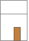
     picturebox[baseline]
     picturebox[baseline] (p1)(p2)
The first form of picturebox causes a scalar baseline
fraction to be emitted in the pspicture
environment of the output. See
PSTricks documentation for pspicture.
In the second form, the baseline fraction is optional, and the
two points that follow define the diagonal of a three-dimensional
bounding box
for the completed scene. The parallel projection
of the bounding box
determines the corners of the drawing's pspicture* environment,
which is used in place of pspicture. This causes PostScript to
clip
the final drawing to the bounding box in 2d. If there is a
camera specified, the camera tranformation is applied to the
bounding box, and the pspicture is set just large
enough to include the transformed box.
When no bounding box is given, sketch computes one
automatically.
frame [options]
Causes a \psframebox
to surround the pspicture
environment in the output. If options are present, they are
copied as-is. Normally one would want to set
linewidth,
linestyle,
linecolor, etc.
If omitted, then
framesep=0pt is
added so that the frame tightly hugs the pspicture.
     language tikz
     language tikz, context
     language pstricks
     language pstricks, latex
Sets the output language generated by sketch.
The set of options understood by sketch also changes. For example,
the PSTricks option linewidth will not be properly
handled if language is set to tikz. Similarly, the
TikZ option line style (note the space) will not be
properly handled if language is set to pstricks. If no
language is specified, the default pstricks is used.
An optional comma followed by
latex
or
context
specifies the macro package that the output should assume. This
affects the picture environment commands emitted and the
document template used with the -T option. See Command line. Note that at the time this manual was generated,
PSTricks was not supported by LaTeX or by ConTeXt.
Successful drawings with sketch and with any scene description
language
require that the user develop an accurate mental picture of her code
and its meaning. This image is best built in small pieces.
Therefore, sketch inputs are best created in small increments
with frequent pauses to compile and view the results. Careful
comments in the input often help as a scene grows in complexity.
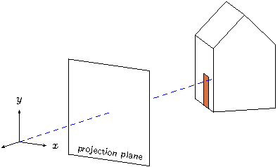
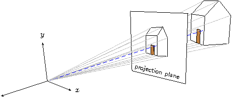
As an overview, let's develop a diagram that shows how a perspective
projection transform
works. We'll start with the traditional reference object
used in computer graphics textbooks, a house-shaped prism. Begin
by defining the points of the house. Rather than defining the faces
of the house as polygons and transforming those, we are going to
transform the points themselves with sketch arithmetic so that
we have names for the transformed points later.
  % right side (outside to right)
  def R1 (1,1,1) def R2 (1,-1,1) def R3 (1,-1,-1) def R4 (1,1,-1)
  def R5 (1,1.5,0)

  % left side (outside to right--backward)
  def W  [2,0,0]
  def L1 (R1)-[W] def L2 (R2)-[W] def L3 (R3)-[W] def L4 (R4)-[W]
  def L5 (R5)-[W]
To add a door to the house, we use a polygon slightly in front of the foremost face of the house.
  % door
  def e .01
  def D1 (0,-1,1+e) def D2 (.5,-1,1+e) def D3 (.5,0,1+e) def D4 (0,0,1+e)
Now let's create a new set of points that are a to-be-determined transform of the originals.
  def hp scale(1) % house positioner
  def pR1 [[hp]]*(R1) def pR2 [[hp]]*(R2) def pR3 [[hp]]*(R3)
  def pR4 [[hp]]*(R4) def pR5 [[hp]]*(R5)
  def pL1 [[hp]]*(L1) def pL2 [[hp]]*(L2) def pL3 [[hp]]*(L3)
  def pL4 [[hp]]*(L4) def pL5 [[hp]]*(L5)
  def pD1 [[hp]]*(D1) def pD2 [[hp]]*(D2) def pD3 [[hp]]*(D3)
  def pD4 [[hp]]*(D4)
Note the use of a transform definition and transform references. Now define the seven polygonal faces of the house and the door using the transformed points as vertices. Be careful with vertex order!
  def rgt polygon (pR1)(pR2)(pR3)(pR4)(pR5)
  def lft polygon (pL5)(pL4)(pL3)(pL2)(pL1)
  def frt polygon (pR2)(pR1)(pL1)(pL2)
  def bck polygon (pR4)(pR3)(pL3)(pL4)
  def tfr polygon (pR1)(pR5)(pL5)(pL1)
  def tbk polygon (pR5)(pR4)(pL4)(pL5)
  def bot polygon (pR2)(pL2)(pL3)(pR3)
  def door polygon[fillcolor=brown] (pD1)(pD2)(pD3)(pD4)
  def house { {rgt}{lft}{frt}{bck}{tfr}{tbk}{bot}{door} }
Time for a sanity check. Add the line
{house}
and this is what we get.
This is correct, but does not reveal very much. Common errors are
misplaced vertices and polygons missing entirely due to incorrect
vertex order.
To rule these out, let's inspect all sides of the
house. This is not hard. Merely replace the reference
{house} with a repeat. See Repeats.
repeat { 13, rotate(30, [1,2,3]), translate([3,0,0]) } {house}
Again things look correct. Note that the hidden surface algorithm handles intersecting polygons correctly where some copies of the house overlap.
Let's lay out the geometry of perspective projection of the house onto a plane with rays passing through the origin. Begin by positioning the house twelve units back on the negative z-axis and adding a set of coordinate axes. To move the house we need only change the “house positioning” transform defined earlier.
  def hp rotate(-40, [0,1,0]) then translate([0,0,-12])
  def axes {
    def sz 1
    line [arrows=<->] (sz,0,0)(O)(0,sz,0)
    line [arrows=->]  (O)(0,0,sz)
    line [linewidth=.2pt,linecolor=blue,linestyle=dashed] (O)(0,0,-10)
    special |\uput[r]#1{$x$}\uput[u]#2{$y$}\uput[l]#3{$z$}|
      (sz,0,0)(0,sz,0)(0,0,sz)
  }
Time for another test. Let's build a real view transform,
creating a virtual camera
to look at the scene we are constructing. Replace the repeat
with
  def eye (10,4,10)
  def look_at (0,0,-5)
  put { view((eye), (look_at)) } { {house}{axes} }
The view transform repositions the scene so that the point
eye is at the origin and the direction from eye to
look_at is the negative z-axis. This requires a
rotation and a translation that are all packed into the constructor
view.
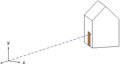
This is starting to look good! Add the projection plane half way
between the origin and the house at z=-5. We'll try
the angle argument feature of special to position a label.
  def p 5 % projection distance (plane at z=-p)
  def projection_plane {
    def sz 1.5
    polygon (-sz,-sz,-p)(sz,-sz,-p)(sz,sz,-p)(-sz,sz,-p)
    special |\rput[b]#1-2#3{\footnotesize\sf projection plane}|
      (-sz,-sz,-p)(sz,-sz,-p)(0,-sz+.1,-p)
  }
Add {projection_plane} to the list of objects in the
put above.
The way we constructed the points of the house now makes it easy to draw rays of projection. We'll cast one ray from every visible vertex of the house and define options so the appearance of all rays can be changed at the same time.
  def projection_rays {
    def rayopt [linewidth=.3pt,linecolor=lightgray]
    line [rayopt](O)(pR1) line [rayopt](O)(pR2) line[rayopt](O)(pR3)
    line [rayopt](O)(pR4) line [rayopt](O)(pR5)
    line [rayopt](O)(pL1) line [rayopt](O)(pL2) line[rayopt](O)(pL5)
    line [rayopt](O)(pD1) line [rayopt](O)(pD2)
    line [rayopt](O)(pD3) line [rayopt](O)(pD4)
  }
The result is shown here.
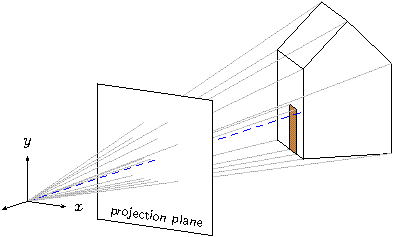
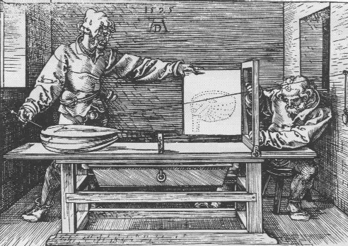
The rays pierce the projection plane at the corresponding points on the perspective image we are trying to draw. Albrecht Dürer and his Renaissance contemporaries had the same idea in the early 1500's.
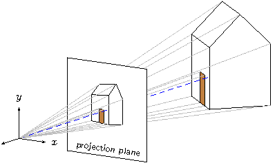
All that's left is to find a way to connect the points of the house
on the projection plane. We could pull out a good computer graphics
text, find the necessary matrix, and enter it ourselves as a
transform literal. See Transform literals. That work is
already done, however. We can use the project(p) constructor.
There are still some details that require care. Projection will flatten whatever is transformed onto the plane z=-p. Therefore any part of the house could disappear behind the projection plane (the hidden surface algorithm orders objects at the same depth arbitrarily). The door may also disappear behind the front of the house. To make sure everything remains visible, we'll place the house a tiny bit in front of the projection plane and a second copy of the door in front of the house.
  def projection {
    % e is a small number defined above
    put { project(p) then translate([0,0,1*e]) } {house}
    put { project(p) then translate([0,0,2*e]) } {door}
  }
If you have studied and understand all this, you are well on the way
to success with sketch. Not shown are the 20 or so iterations
that were required to find a reasonable viewing angle and house
position, etc. Nonetheless, this drawing was completed in about an
hour. While a GUI tool may have been a little faster, it is unlikely
that a new drawing, itself a perspective projection of the scene,
could be generated with two more minutes' work! Just change the view
transform to
put { view((eye), (look_at)) then perspective(9) } { ...
and produce this.
Let's look at a drawing that represents the kind of problem
sketch was meant to solve—a pair of textbook figures
regarding a polygonal approximation of a truncated cone. Here are the
pictures we will produce.
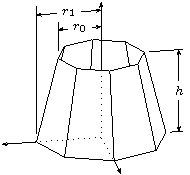
The cone shape is just a swept line with no closure tag and culling turned off. Begin by setting up some useful constants.
  def O (0,0,0) def I [1,0,0] def J [0,1,0] def K [0,0,1]
  def p0 (1,2) def p1 (1.5,0) def N 8
  def seg_rot rotate(360 / N, [J])
The points
p0 and p1 are the end points of the line to
be swept. The definition seg_rot is the sweep transformation.
With these, the cone itself is simple.
sweep[cull=false] { N, [[seg_rot]] } line(p0)(p1)
The axes are next and include an interesing trick that shows the
hidden parts as dotted lines. The secret is draw the axes
twice—solid lines with the normal
hidden surface algorithm in effect, and then dotted with the
option
lay=over so that no polygons can hide them.
  def ax (dx,0,0) % tips of the axes
  def ay (0,dy,0)
  def az (0,0,dz)
  line[arrows=<->,linewidth=.4pt](ax)(O)(ay)
  line[arrows=->,linewidth=.4pt](O)(az)
  % repeat dotted as an overlay to hint at the hidden lines
  line[lay=over,linestyle=dotted,linewidth=.4pt](ax)(O)(ay)
  line[lay=over,linestyle=dotted,linewidth=.4pt](O)(az)
  special|\footnotesize
          \uput[d]#1{$x$}\uput[u]#2{$y$}\uput[l]#3{$z$}|
    (ax)(ay)(az)
The labels are applied with PSTricks special objects
as usual.
For the height dimension mark, the power of affine arithetic is very helpful.
  def hdim_ref unit((p1) - (O)) then [[seg_rot]]^2
  def c0 (p0) then scale([J])
  def h00 (c0) + 1.1 * [hdim_ref]
  def h01 (c0) + 1.9 * [hdim_ref]
  def h02 (c0) + 1.8 * [hdim_ref]
  line(h00)(h01)
  def h10 (O) + 1.6 * [hdim_ref]
  def h11 (O) + 1.9 * [hdim_ref]
  def h12 (O) + 1.8 * [hdim_ref]
  line(h10)(h11)
  line[arrows=<->](h02)(h12)
  def hm2 ((h02) - (O) + (h12) - (O)) / 2 + (O)
  special|\footnotesize\rput*#1{$h$}|(hm2)
The general idea employed here is to compute a unit “reference
vector” parallel to the xz-plane in the desired direction of
the dimension from the origin. The transformation
[[seg_rot]]^2 rotates two segments about the y-axis.
When applied to (p1) - (O), the resulting vector points to the
right as shown. In this manner, we can pick any vertex as the
location of the height dimension lines by varying the exponent of
[[seg_rot]]. This is only one of many possible strategies.
The computation of hm2 is a useful idiom for finding the
centroid of a set of points.
The two radius marks are done similarly, so we present the code without comment.
  % radius measurement marks
  def gap [0,.2,0]  % used to create small vertical gaps

  % first r1
  def up1 [0,3.1,0] % tick rises above dimension a little
  def r1 ((p1) then [[seg_rot]]^-2) + [up1]
  def r1c (r1) then scale([J])
  def r1t (r1) + [gap]
  def r1b ((r1t) then scale([1,0,1])) + [gap]
  line[arrows=<->](r1c)(r1)  % dimension line
  line(r1b)(r1t)             % tick
  def r1m ((r1) - (O) + (r1c) - (O)) / 2 + (O) % label position
  special |\footnotesize\rput*#1{$r_1$}|(r1m)  % label

  % same drill for r0, but must project down first
  def up0 [0,2.7,0]
  def r0 ((p0) then scale([1,0,1]) then [[seg_rot]]^-2) + [up0]
  def r0c (r0) then scale([J])
  def r0t (r0) + [gap]
  def r0b ((p0) then [[seg_rot]]^-2) + [gap]
  line[arrows=<->](r0c)(r0)
  line(r0b)(r0t)
  def r0m ((r0) - (O) + (r0c) - (O)) / 2 + (O)
  special |\footnotesize\rput*#1{$r_0$}|(r0m)
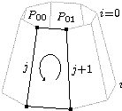
The second drawing uses the same techniques. Only the method for drawing the elliptical arc is new. Here is the code.
  def mid ((p00)-(O)+(p10)-(O)+(p11)-(O)+(p01)-(O))/4+(O)
  special|\rput#1{\pscustom{
    \scale{1 1.3}
    \psarc[arrowlength=.5]{->}{.25}{-60}{240}}}|
    [lay=over](mid)
We could have swept a point to make the arc with sketch, but
using a PSTricks custom graphic was simpler. Again we computed
the
centroid of the quadrilateral by averaging points. Note that scaling
in Postscript distorts the arrowhead, but in this case the distortion
actually looks better in the projection of the slanted face. A
sketch arrowhead would not have been distorted.
The complete code for this example, which draws either figure
depending on the definition of the tag <labeled>, is included
in the sketch distribution in the file truncatedcone.sk.
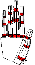
While sketch was never meant to be a geometric modeling
language, it comes fairly close. The following example puts all we
have seen to work in a very simple model of the human hand. Start by
sweeping a line to make a truncated cone, which will be copied over
and over again to make the segments of fingers.
  def O (0,0,0) % origin
  def I [1,0,0] def J [0,1,0] def K [0,0,1] % canonical unit vectors
  def segment {
    def n_faces 8
    sweep { n_faces<>, rotate(360 / n_faces, [J]) }
      line(proximal_rad, 0)(distal_rad, distal_len)
  }
In hand anatomy, distal is “at the tip” and proximal
is “in the area of the palm.” We have omitted all the scalar
constants. You can find them in hand.sk, which is provided
in the sketch distribution.
We also need a prototypical sphere to use for the joints themselves.
  def joint_sphere {
    def n_joint_faces 8
    sweep [fillcolor=red] { n_joint_faces, rotate(360 / n_joint_faces, [J]) }
      sweep { n_joint_faces, rotate(180 / n_joint_faces) }
        (0, -joint_rad)
  }
We'll now design the index finger (number 1 in our notational convention; finger 0 is the thumb). The distal rotation for the finger applies only to the tip, so we define the following.
  def distal_1 {
    put { translate(joint_gap * joint_rad * [J])
          then rotate(distal_1_rot, [I])
          then translate((distal_len + joint_gap * joint_rad) * [J]) }
      {segment}
    put { rotate(distal_1_rot / 2, [I])
          then translate((distal_len + joint_gap * joint_rad) * [J]) }
      {joint_sphere}
    put { scale( [J] + proximal_distal_ratio * ([I]+[K]) ) }
      {segment}
  }
The identifiers here are for size and location constants. The
exception is distal_rot_1. This rotation parameter models the
flexing of the finger tip. The first put makes a copy of the
finger segment that is translated upward
just far enough to make room
for the spherical joint. Then it applies the distal rotation.
Finally it translates the whole assembly upward again to make room for
the middle phlanges (the next bone toward the palm). The second
put positions the sphere. There is a rotation to place the
grid on the sphere surface at an nice angle, then a translation to the
base of the distal phlanges, which is also center of its rotation.
Finally, the last put positions the middle segment itself.
The middle joint is the next one down, with rotation angle
middle_rot_1. When this angle changes, we need all the objects
in distal_1 to rotate as a unit.
This is the reasoning behind
the next definition.
  def finger_1 {
    put { translate(joint_gap * joint_rad * [J])
          then rotate(middle_1_rot, [I])
          then translate((middle_ratio * distal_len +
                          joint_gap * joint_rad) * [J]) }
      {distal_1}
    put { scale(proximal_distal_ratio)
          then rotate(middle_1_rot / 2, [I])
          then translate((middle_ratio * distal_len +
                          joint_gap * joint_rad) * [J]) }
      {joint_sphere}
    put { scale( middle_ratio * [J] +
                 proximal_distal_ratio^2 * ([I]+[K]) ) }
      {segment}
  }
This looks very similar to the previous definition, and it is. The
important difference is that rather than positioning and rotating a
single segment, we position and rotate the entire “assembly” defined
as distal_1.
The rest is just arithmetic to compute sizes and
positions that look nice. The last put places an appropriately
shaped segment that is the proximal phlanges, the bone that
joins the palm of the hand. This completes the finger itself.
All the other fingers are described identically to this one. We account for the fact that real fingers are different sizes in the next step, which is to build the entire hand.
The hand definition that follows includes a section for each
finger. We'll continue with finger 1 and omit all the others.
(Of note is that the thumb needs slightly special treatment—an extra
rotation to account for its opposing angle. This is clear in the full
source code.) Not surprisingly, the hand definition looks very
much like the previous two. It should be no surprise that when the
rotation parameter meta_1_rot changes, the entire finger
rotates!
There is an additional rotation that allows the fingers to spread
laterally. We say these joints of the proximal phlanges have two
degrees of freedom. The joints higher on the finger have only
one. Finally, each finger is scaled by a factor to lend it proportion.
  def hand {
    % finger 1 [all other fingers omitted]
    def scale_1 .85
    put { scale(scale_1)
          then translate((joint_gap * joint_rad) * [J])
	  then rotate(meta_1_rot, [I])
          then rotate(-spread_rot, [K])
          then translate((proximal_1_loc) - (O)) }
      {finger_1}
    put { scale(scale_1 * proximal_distal_ratio^2)
          then rotate(meta_1_rot / 2, [I])
          then rotate(-spread_rot, [K])
          then translate((proximal_1_loc) - (O)) }
      {joint_sphere}

    % palm
    sweep { 1, rotate(6, (0,15,0), [I]) }
      put { rotate(-3, (0,15,0), [I]) } {
        polygon(proximal_1_loc)(proximal_2_loc)
               (proximal_3_loc)(proximal_4_loc)
               (h5)(h6)(h6a)(h9)(h10)
        polygon(h6a)(h7)(h8)(h9)
   }  }
The last section of the definition creates the polytope for the palm
of the hand by sweeping
a 10-sided polygon through a very short
arc (9 degrees). This provides a wedge-shaped profile when viewed
from the side. The thick end of the wedge is the wrist. Because the
polygon is concave, it is split into into two convex shapes with nine
and four vertices.
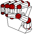
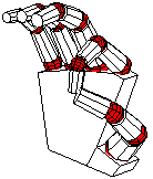
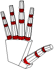
We can now have fun positioning the hand by adjusting the various rotation angles. The complete source includes definitions with alternatives that include the following views and more.
Sketch is a fairly powerful tool for drawing, but, just as with
TeX, the power to create beautiful results comes along with the
power to make mistakes. The following are some points where care is
necessary and where the current version of sketch is limited or
has known bugs.
sketch error detectionSketch catches many kinds of errors, but not all. For example,
options that sketch does not recognize, even incorrect ones, are
quietly copied to PSTricks commands in the output. It is also
unfortunately easy to produce sketch inputs that lead to no
picture at all (improper vertex ordering causes everything to be
culled), to pictures that are too big or too small for PSTricks
to draw (due to limits of TeX math), and pictures that look nothing
like what was intended. A picture with one of these problems can be
difficult to “debug.” We offer the following suggestions.
perspective, ensure all finally transformed objects
satisfy z<0 and, in fact, do not come very close to the origin
at all.
cull=false to see where vertex ordering
problems lie.
PSTricks complains about something, inspect the output
directly for clues.
The current version of sketch has no clipping
operations. The entire scene is always drawn. This means that when a
perspective transform is employed, it is the user's responsibility to
make sure the entire scene remains in front of the viewer, the region
z<0.
Sketch uses the depth sort algorithm
for hidden surface removal. This is a very old technique due to
Newell.3 It is
generally regarded as too slow for real time graphics, but it is
ideal for our purpose where speed is not very important.4
The depth sort algorithm merely sorts objects on a key of increasing z-coordinate, equivalent to decreasing depth. Objects are then drawn in the sorted sequence so that those at the rear of the scene are overwritten by those closer to the viewer. Since this is also how oil painters practice their art, depth sort is sometimes called “the painter's algorithm.”
In some cases it is impossible to strictly order polygons according to
depth. Moreover, even if a correct depth ordering exists, the
computation needed to find it may be too complex and slow. In these
cases, sketch splits
one or more polygons into pieces. The
expectation is that the new, smaller polygons will be simpler to
order. Sketch uses a BSP (binary space partition)
to handle the splitting operation.
For the curious, sketch writes one line of depth sort
statistics. Here is an example for a large collection of triangles.
remark, node=34824 probe=581.9 swap=5 split=2 (in=4 out=6) ols=24851/0It means that 34,824 objects were depth sorted after culling. For each, an average of 581.9 others had to be checked to ensure that the initial, approximate ordering was correct. Among all these checks, only 5 resulted in swaps to reorder the initial sort. In two cases, a correct ordering could not be determined, so binary space partitions were constructed for splitting. A total of 4 objects (triangles in this case) were inserted in the partitions, and 6 polygons were produced. Finally, 24,851 “last resort” polygon overlap checks were performed after simpler, faster checks failed to yield conclusive results. The final /0 is for line-polygon overlap checks. For comparison, the statistics for the last figure in Overview follow.
remark, node=27 probe=14.6 swap=36 split=15 (in=30 out=45) ols=0/69Note that there was proportionally much more swapping and splitting activity in this highly connected scene.
Polygon and line splitting can both cause anomalies in the output.
PSTricks dash patterns, specified with linestyle=dashed,
can be disrupted by splitting. This occurs when the depth sort
gives up too early and splits a line where it is not really
necessary.
A workaround is to use gray or finely dotted
lines instead. If your drawing is small, you can also edit the
sketch output by hand to merge the pieces of the offending
line.
Another anomaly is tiny (or in degenerate cases not-so-tiny) notches
in the lines that border split polygons. These derive from the way
each polygon is painted: first, all pixels within the boundary are
filled with color (perhaps white), then the same boundary is
stroked (a Postscript term) with a line. The result is that
half the line lies inside the boundary and half outside, while the
Painter's algorithm assumes the polygon lies entirely within its
boundary. The notches are due to one polygon fill operation
overwriting the already-drawn inside of the border of another
polygon.5 One workaround is to make
border lines very thin. In fact linewidth=0pt is guaranteed to
eliminate this problem, though this results in the thinnest line your
output device can draw, which is usually too thin. You might get
lucky by merely reordering things in the input file, which is likely
to move the splits to different places. The only sure-fire solution
is pretty terrible: custom fit special overlay lines (with
\psline) to cover the notches.
Polygon splitting also breaks PSTricks hatch patterns. The
only known workaround is to substitute a solid fill for the hatch.
     sketch [-h][-V x.y][-v][-b][-d][t doctmp][-T[u|e][p[P|T][L|C]]][-o output.tex]
       [-D tag ...] input1.sk [-U tag ...] input2.sk ...
Description
Processes the sketch input files in order to produce
PSTricks output code suitable for inclusion in a TeX or
LaTeX document.
-h-VPSTricks version assumed for output purposes to
x.y, for example 1.19. Usually needed only if your
PSTricks is old compared to your sketch. Use
-v to see what sketch assumes by default.
-vPSTricks assumed for output (can be changed with -V above).
-b-dsketch's parser in debugging mode. This is primarily for
development.
-tPSTricks output code. The code is inserted
in place of the first instance of the escape string
%%SKETCH_OUTPUT%%.
-TPSTricks output to be enclosed in default US document
template text. Option -Tu is a synonym. Option -Te
causes the Euro standard document template to be used. A p
appended to any of these options causes the respective default
PSTricks document template to be printed to standard output. An
appended P is a synonym. An appended T causes the
the TikZ/PGF template to be printed. An appended L
prints the LaTeX version of the document template, a synonym for
the default. A C prints the ConTeXt template.
-o-Dinputi.sk-UsketchSketch is so small that compiling by brute force is probably
best. The following command ought to do the trick on any
systems where gcc is installed. Make sure to first change
current directories to the place where you have unpacked the sources.
gcc *.c -o sketch.exe -lm
The .exe at the end is necessary for Windows systems. Drop it if your system is some version of Unix. Other C compilers ought to work as just as well. For example,
cl *.c -o sketch.exe
is the correct command for many versions of MS Visual C. In the
latest versions, Microsoft has deprecated the -o option and, by
default, does not define the __STDC__ macro. This causes
problems with some versions of flex, bison, lex,
and yacc, which are used to create the sketch scanner
and parser. It's nearly always possible to find a set of options that
compiles with no errors or warnings, and this means sketch is
very likely to work correctly. For example, the Visual C++
2005 Express Edition compiler (available free of charge from the
Microsoft web site), flex version 2.5.4, and bison
version 2.1 build error-free with
cl -DYY_NEVER_INTERACTIVE=1 -Za -Ox -Fesketch.exe *.c
For purists, there is also a makefile compatible with GNU
make and gcc. The command
make
will build the executable, including the rebuilding of the scanner and
parser with flex and bison if you have changed
sketch.l or sketch.y respectively.
To build this document in all its myriad forms (assuming you have the necessary conversion programs on your system), use
make docs
The possibilities are listed in this following table.
| Format | Converter | Pictures | Description
|
|---|---|---|---|
| manual.info | makeinfo | .txt | GNU Info.
|
| manual.dvi | texi2dvi | .eps | TeX typeset output.
|
| manual.ps | texi2dvi,dvips | .eps | Postscript.
|
| manual.pdf | texi2dvi | Adobe PDF.
| |
| manual.html | makeinfo | .png | A single web page.
|
| manual/index.html | makeinfo | .png | Linked web pages, one per node.
|
'x, 'y, and 'z: Two-operand (binary) forms'x, 'y, and 'z: Affine arithmetic( ), grouping: Two-operand (binary) forms(foo), point reference: Forms of references(foo), point reference: Drawing a solid*, multiplication operator: Two-operand (binary) forms+, plus operator: Two-operand (binary) forms-, minus operator: Two-operand (binary) forms-, unary minus operator: Unary forms., dot operator: Two-operand (binary) forms/, division operator: Two-operand (binary) forms<>, closure tag: Swept lines<>, closure tag: Sweep face splitting<>, closure tag: Swept lines<>, closure tag: Polyline sweeps with closure<>, closure tag: Point sweeps<>, closure tag: Sweeps<>, closure tag: Swept points<foo>, tag reference: Forms of definitions<foo>, tag reference: Forms of references[[ ][ ][ ][ ]], transform literal: Transform literals[[foo]], transform reference: Overview[[foo]], transform reference: Forms of references[[foo]], transform reference: Overview[foo,...,bar], multiple options reference: Forms of references[foo], options reference: Forms of references[foo], options reference: Polyline sweeps with closure[foo], vector reference: Forms of references[foo], vector reference: Polyline sweeps^, exponentiation operator: Two-operand (binary) formsarrows: Affine arithmeticarrows: A technical drawingarrows: Overviewarrows: A technical drawingatan2: Unary formscamera: Cameracontext: Languagecos: Unary formscull: Internal optionscull: A technical drawingcull: Drawing a solidcull: Transparencycull: Polyline sweepscull: Global optionscurve: Curvesdef: Affine arithmeticdef: Overviewdef: Polyline sweepsdef: Drawing a soliddef: A hierarchical modeldef: Overviewdef: A hierarchical modeldef: Object transformsdef: A hierarchical modeldef: Overviewdef: A technical drawingdef: Polyline sweeps with closuredef: A technical drawingdef: Point sweepsdef: Nested sweepsdef: A technical drawingdots: Dotsfill opacity: Transparencyfill style: TikZ/PGF user-defined stylesfillcolor: Object transformsfillcolor: Overviewfillcolor: Polyline sweeps with closureframe: Frameframesep: Frameglobal: Global environmentinput: Language basicsinverse: Unary formslanguage: Languagelatex: Languagelay: Specialslay: Global optionslay: Internal optionslay: Special objectslay: A technical drawingline: Object transformsline: Overviewline: Swept blocksline: A hierarchical modelline: Linesline: Drawing optionsline: A technical drawingline: Polyline sweeps with closureline: A technical drawingline: Affine arithmeticline style: TikZ/PGF user-defined styleslinecolor: Framelinecolor: Object transformslinecolor: Overviewlinestyle: A technical drawinglinestyle: Framelinestyle: Bugs and anomalieslinestyle: Overviewlinewidth: Framelinewidth: Polyline sweepslinewidth: A technical drawinglinewidth: Overviewopacity: Transparencyperspective: Transform literalspicturebox: Picture boxpoint list: Internal optionspolygon: Polygonspolygon: Swept blockspolygon: Drawing a solidpolygon: Hello worldpolygon: Overviewpolygon: Affine arithmeticpolygon: Object transformsproject: Transform literalspstricks: Languageput: Nested sweepsput: Putsput: Object transformsput: A hierarchical modelrepeat: Nested sweepsrepeat: Repeatsrepeat: Polyline sweeps with closurerepeat: Overviewrepeat: Repeated objectsrotate: Object transformsrotate: A hierarchical modelrotate: A technical drawingrotate: A hierarchical modelrotate: Polyline sweeps with closurerotate: Polyline sweepsrotate: Repeated objectsrotate: Transform literalsrotate: Swept objectsrotate: Point sweepsrotate: Overviewrotate: A hierarchical modelrotate: Nested sweepsscale: A hierarchical modelscale: A technical drawingscale: Transform literalsscale: A technical drawingset: Global optionssin: Unary formsspecial: Special objectsspecial: Specialsspecial: A technical drawingspecial: Overviewspecial: A technical drawingsplit: Internal optionssplit: Global optionssqrt: Unary formssweep: Sweepssweep: A technical drawingsweep: Nested sweepssweep: A hierarchical modelsweep: Polyline sweepssweep: Polyline sweeps with closuresweep: Point sweepssweep: Swept objectsthen: Object transformsthen: Polyline sweeps with closurethen: Two-operand (binary) formstikz: Languagetranslate: Transform literalstranslate: A hierarchical modeltranslate: Object transformstranslate: Polyline sweepstranslate: Polyline sweeps with closuretranslate: Overviewtranslate: Object transformstranslate: Repeated objectstranspalpha: Transparencyunit: A technical drawingunit: Unary formsview: Transform literals{ }, block drawable: Overview{ }, block drawable: Swept blocks{ }, block drawable: Blocks{ }, block drawable: Object transforms{ }, block drawable: Nested sweeps{foo}, drawable reference: Overview{foo}, drawable reference: Forms of references{foo}, drawable reference: Overview{foo}, drawable reference: Object transforms|X|, magnitude operator: Unary forms<>: Swept points<>: Point sweeps<>: Swept lines<>: Polyline sweeps with closure<>: Sweeps<>: Swept points<>: Swept lines<>: Sweep face splittingsketch: Hello worldsketch: Command linepsframebox: Framepspicture: Picture boxsketch: Hello world'): Affine arithmetic'): Two-operand (binary) forms[1] Or for European users of A4 size paper, -Te.
[2] This clever trick is due to Kjell Magne Fauske.
[3] Newell, M.E., R.G. Newell, and T.L. Sancha, A solution to the hidden surface problem. Proceedings of the ACM annual conference - Volume 1, page 443–450, ACM Press, 1972.
[4] We
have run sketch on the famous Stanford Bunny, which consists
of nearly 70,000 triangles. Run time was about 6 seconds.
Most of this was spent writing the output file rather than in the
hidden surface algorithm. LaTeX took much longer to process the
resulting PSTricks code. The obvious conclusion is that the
speed of the depth sort algorithm is not a worry.
[5] I know how to fix this problem, but I don't like my solution, and I'm interested in yours.